Quick wordclouds from PubMed abstracts – using PMID lists in R

Posted on septiembre 26, 2016 por mareviv

Wordclouds are one of the most visually straightforward, compelling ways of displaying text info in a graph.

Of course, we have a lot of web pages (and even apps) that, given an input text, will plot you some nice tagclouds. However, when you need reproducible results, or getting done complex tasks -like combined wordclouds from several files-, a programming environment may be the best option.

In R, there are (as always), several alternatives to get this done, such as tagcloud and wordcloud.

For this script I used the following packages:

«RCurl» to retrieve a PMID list, stored in my GitHub account as a .csv file.
«RefManageR» and «plyr« to retrieve and arrange PM records. To fetch the info from the inets, we’ll be using the PubMed API (free version, with some limitations).
Finally, «tm«, «SnowballC» to prepare the data and «wordcloud» to plot the wordcloud. This part of the script is based on this from Georeferenced.

One of the advantages of using RefManageR is that you can easily change the field which you are importing from, and it usually works flawlessly with the PubMed API.

My biggest problem sources when running this script: download caps, busy hours, and firewalls!.

At the beginning of the gist, there is also a handy function that automagically downloads all needed packages for you.

To source the script, simply type in the R console:

This script creates two directories in your working directory: ‘corpus1‘ for the abstracts file, and ‘wordcloud‘ to store the plot.

library(devtools)
source_url("https://gist.githubusercontent.com/aurora-mareviv/697cbb505189591648224ed640e70fb1/raw/b42ac2e361ede770e118f217494d70c332a64ef8/pmid.tagcloud.R")

And there is the code:

	#########################################################
	#### CAPTURE ABSTRACTS FROM PMIDs & MAKE A WORDCLOUD ####
	#########################################################

	# GNU-GPL license
	# Author: Mareviv (https://talesofr.wordpress.com)

	# Script to retrieve and mine abstracts from PubMed (http://www.ncbi.nlm.nih.gov/pubmed)
	# Uses the function ReadPubMed from the package RefManageR. It reads the PubMed API similarly to the search engine in PubMed's page.
	# This script creates two directories in your working directory: 'corpus1' for the abstracts file, and 'wordcloud' to store the plot.

	# First, automagically install needed libraries:
	list.of.packages <- c("slam") # installing 'slam' gives error in OSX Yosemite/El Capitan. This is an attempt to fix it, specifying 'type="binary"'.
	new.packages <- list.of.packages[!(list.of.packages %in% installed.packages()[,"Package"])]
	if(length(new.packages)) install.packages(new.packages, repos='https://cran.rstudio.com/', type="binary")

	list.of.packages <- c("RCurl", "RefManageR", "plyr", "tm", "wordcloud", "SnowballC")
	new.packages <- list.of.packages[!(list.of.packages %in% installed.packages()[,"Package"])]
	if(length(new.packages)) install.packages(new.packages, repos='https://cran.rstudio.com/')

	# Get and store the working directory
	wdir <- getwd()


	# 1. Import PMIDs
	message("retrieving PMIDs info…")
	library(RCurl)
	urli <- getURL("https://gist.githubusercontent.com/aurora-mareviv/14e5837814a8d8d47c20/raw/90b198bae82154688dcd9a2596af798612e6619f/pmids.csv", ssl.verifypeer = FALSE)
	pmids <- read.csv(textConnection(urli))
	message("PMID info succesfully retrieved")


	# 2. Loop several queries to PubMed and return in a data.frame
	index <- pmids$pmId[1:length(pmids$pmId)]
	# The PubMed (free) API may give problems with large queries, so we'll prefer a shorter vector for this test:
	index50 <- pmids$pmId[1:50]

	library(RefManageR)
	library(plyr)
	message("connecting to the free PubMed API…")
	auth.pm <- ldply(index50, function(x){
	tmp <- unlist(ReadPubMed(x, database = "PubMed", mindate = 1950))
	tmp <- lapply(tmp, function(z) if(is(z, "person")) paste0(z, collapse = ",") else z)
	data.frame(tmp, stringsAsFactors = FALSE)
	})
	message("abstract data successfully downloaded!")


	# 3. Create a directory to write the abstracts.txt file into: (this folder can only contain this .txt file!)
	corpus.dir <- paste(wdir, "corpus1", sep="/")
	message(paste("creating new directory: ", corpus.dir, sep=""))
	dir.create(corpus.dir)
	setwd(corpus.dir)


	# 4. Extract abstracts to a .txt
	text <- paste(auth.pm$abstract)
	message(paste("writing file: ", corpus.dir, "/abstracts.txt", sep=""))
	writeLines(text, "abstracts.txt")


	# 5. Create tagcloud
	library(tm)
	library(wordcloud)
	library(SnowballC)

	message("constructing the tagcloud…")
	abstract <- Corpus (DirSource(corpus.dir)) # import text file in this directory
	abstract <- tm_map(abstract, stripWhitespace) # transformations
	abstract <- tm_map(abstract, content_transformer(tolower))
	abstract <- tm_map(abstract, removeWords, stopwords("english"))
	# abstract <- tm_map(abstract, stemDocument) # optional in this case
	abstract <- tm_map(abstract, removeNumbers) # optional in this case
	abstract <- tm_map(abstract, removePunctuation)
	# tuning
	abstract <- tm_map(abstract, removeWords, "methods")
	abstract <- tm_map(abstract, removeWords, "results")
	abstract <- tm_map(abstract, removeWords, "conclusions")
	abstract <- tm_map(abstract, removeWords, "conclusion")
	abstract <- tm_map(abstract, removeWords, "whether")
	abstract <- tm_map(abstract, removeWords, "due")


	# 6. Print image in a new folder: wordcloud
	plot.dir <- paste(wdir, "wordcloud", sep="/")
	message(paste("creating new directory: ", plot.dir, sep=""))
	dir.create(plot.dir)
	setwd(plot.dir)
	message(paste("printing file: ", plot.dir, "/wordcloud.png", sep=""))
	png(file = "wordcloud.png", width = 1500, height = 1500, units = "px", res = 300, bg = "transparent")
	wordcloud(abstract, scale=c(5,0.5), max.words=150, random.order=FALSE, rot.per=0.35, use.r.layout=FALSE, colors=brewer.pal(8, "Dark2"))
	dev.off()


	# 7. Reset the working directory
	setwd(wdir)

view raw

pmid.tagcloud.R

hosted with ❤ by GitHub

Enjoy!

wordcloud

R/Shiny for clinical trials: simple randomization tables

Posted on junio 9, 2016 por mareviv

One of the things I most like from R + Shiny is that it enables me to serve the power and flexibility of R in small «chunks» to cover different needs, allowing people not used to R to benefit from it. However, what I like most is that’s really fun and easy to program those utilities for a person without any specific programming background.

Here’s a small hack done in R/Shiny: it covered an urgent need for a study involving patient randomisation to two branches of treatment, in what is commonly known as a clinical trial. This task posed some challenges:

First, this trial was not financed in any way (at least initially). It was a small, independent study comparing two approved techniques for chronic pain, so the sponsor had to avoid expensive software or services.
Another reason for software customization is that treatment groups were partially ‘blind’: for people who assessed effectiveness and… also for statistical analysis (treatment administration was open-label). This means that the person in charge of data analysis must know which group is assigned to a patient, but doesn’t know what treatment is assigned to either group.

To tackle the points above, my app should have two main features:

The sponsor (here, a medical doctor) must be able to effectively control study blindness and also provide emergency blind disclosure. This control should extend to data analysis to minimize bias favoring either treatment.
R has tools to create random samples, but the MD in charge of the study sponsoring doesn’t know how to use R. We needed a friendly interface for random table creation.

Here’s how I got it to work:

The very core of this Shiny app is a combination between the set.seed and sample R functions. The PIN number (the set.seed argument) works like a secret passcode that links to a given random table. E.g., every time I enter ‘5432’, the random tables will look the same. This protects from accidental blindness disclosure, as nobody can find the correct random table without the proper PIN, even if they can access the app’s source code.
The tables are created column by column, ordered at first. Then we proceed to randomize (via the sample function) both the treatment column (in the random table) and the Group column (in the PIN table).
Once the tables are created they can be downloaded as .CSV files, printed, signed and dated to document the randomization procedure. The app’s open source code and the PIN number will provide reproducibility to the procedure for many years.

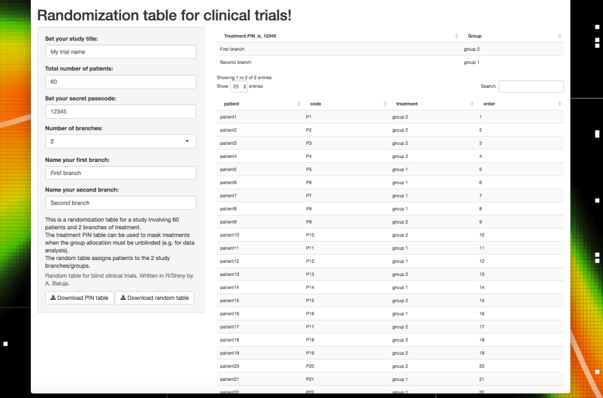
Unfortunately I wasn’t able to insert iframes to embed the app, so I posted a screenshot:

Random table generator for clinical trials

The app is far from perfect, but it covers the basic needs for the trial. You can test it here:

http://aurora.shinyapps.io/random_gen

And the GitHub repo is available here. Feel free to use/ adapt/ fork it to your needs!

https://github.com/aurora-mareviv/random_gen

Also, you can cite it if it’s been useful for your study methods!

	# server.R

	shinyServer(function(input, output) {

	f <- function(seed, ncases, branches){
	set.seed(seed)
	branch <- branches
	if(branch==2){ # table creation
	rond1 <- round(ncases/2, 0)
	rond2 <- ncases-rond1

	patient <- seq(1:ncases)
	code <- paste("P", patient, sep="")
	patient <- paste("patient", patient, sep="")
	treatment <- c(rep("group 1", rond1), rep("group 2", rond2))
	order <- seq(1:ncases)
	}
	if(branch==3){ # table creation
	rond1 <- round(ncases/3, 0)
	rond2 <- rond1
	rond3 <- ncases-(rond1+rond2)
	patient <- seq(1:ncases)
	code <- paste("P", patient, sep="")
	patient <- paste("patient", patient, sep="")
	treatment <- c(rep("group 1", rond1), rep("group 2", rond2), rep("group 3", rond3))
	order <- seq(1:ncases)
	}
	random.0 <- data.frame(patient, code, treatment, order)
	random.1 <- transform(random.0, treatment = sample(treatment)) # here goes the randomisation (sampling the treatment column)
	random.1
	}

	g <- function(seed, branches){
	set.seed(seed)
	branch <- branches
	if(branch==2){ # table creation
	Treatment.Key <- c(paste(input$tta), paste(input$ttb))
	Group <- c("group 1", "group 2")
	}
	if(branch==3){ # table creation
	Treatment.Key <- c(paste(input$tta), paste(input$ttb), paste(input$ttc))
	Group <- c("group 1", "group 2", "group 3")
	}
	chave <- data.frame(Treatment.Key, Group)
	chave.rand <- transform(chave, Group = sample(Group)) # here goes the randomisation (sampling the Group column)
	names(chave.rand)[1] <- paste("Treatment.PIN_is_", seed, sep="")
	chave.rand
	}


	mydata <- reactive(f(input$seed,
	input$ncases,
	input$branches))

	mydatachave <- reactive(g(input$seed,
	input$branches))

	# Show the final calculated values from RAND table

	output$randTable <- renderDataTable(
	{mydata <- f(input$seed,
	input$ncases,
	input$branches)
	mydata}
	)

	output$randChave <- renderDataTable(
	{mydatachave <- g(input$seed,
	input$branches)
	mydatachave},
	options = list(searching = FALSE, paging = FALSE, caption = 'Table 1: This is it')
	)

	output$text1 <- renderText({
	paste("This is a randomization table for a study involving ",
	input$ncases,
	" patients and ",
	input$branches,
	" branches of treatment.",
	sep="")
	})

	output$text2 <- renderText({
	paste("- The treatment PIN table can be used to mask treatments when the group allocation must be unblinded (e.g. for data analysis).",
	sep="")
	})

	output$text3 <- renderText({
	paste("- The random table assigns patients to the ", input$branches, " branches/groups.",
	sep="")
	})

	info <- sessionInfo()
	output$version <- renderText({
	paste(info$R.version[c(13, 2)]$version.string, info$R.version[c(13, 2)]$arch,
	sep=", ")
	})

	output$downloadChave <- downloadHandler(
	filename = function() { paste(input$title, 'treatment_allocation_PIN.csv', sep='-') },
	content = function(file) {
	write.csv(mydatachave(), file, na="")
	}
	)

	output$downloadData <- downloadHandler(
	filename = function() { paste(input$title, 'random_table.csv', sep='-') },
	content = function(file) {
	write.csv(mydata(), file, na="")
	}
	)


	})

view raw

server.R

hosted with ❤ by GitHub

	# ui.R

	library(shiny)

	# Define UI for slider demo application
	shinyUI(pageWithSidebar(

	# Application title
	headerPanel("Randomization table for clinical trials!"),

	# Sidebar with sliders that demonstrate various available options
	sidebarPanel(
	# Simple integer interval
	textInput("title", "Set your study title:", "My trial name"),
	numericInput("ncases", label = "Total number of patients:", value = 60),
	numericInput("seed", label = "Set your secret passcode:", value = 12345),
	selectInput("branches", "Number of branches:",
	choices = c("2", "3")),
	textInput("tta", "Name your first branch:", "First branch"),
	textInput("ttb", "Name your second branch:", "Second branch"),
	conditionalPanel(
	condition = "input.branches == 3",
	textInput("ttc", "Name your third branch:", "Third branch")),
	textOutput("text1"),
	textOutput("text2"),
	textOutput("text3"),
	textOutput("version"),
	helpText("Random table for blind clinical trials.
	Written in R/Shiny by A. Baluja."),
	downloadButton('downloadChave', 'Download PIN table'),
	downloadButton('downloadData', 'Download random table')
	),

	# Show a table summarizing the values entered
	mainPanel(
	div(dataTableOutput("randChave"), style = "font-size:80%"),
	div(dataTableOutput("randTable"), style = "font-size:80%")
	)
	)
	)

	# To execute this script from inside R, you need to have the ui.R and server.R files into the session's working directory. Then, type:
	# runApp()
	# To execute directly this Gist, from the Internet to your browser, type:
	# shiny:: runGist(' ')

view raw

ui.R

hosted with ❤ by GitHub

Install R in Android, via GNURoot -no root required!

Posted on septiembre 30, 2014 por mareviv

Playing with my tablet some time ago, I wondered if installing R could be possible. You know, a small android device «to the power of R»…

After searching on Google from time to time, I came across some interesting possibilities:

R Instructor, created «to bridge the gap between authoritative (but expensive) reference textbooks and free but often technical and difficult to understand help files«.
R Console Free. provides the necessary C, C++ and Fortran compilers to build and install R packages.
There’s always possible to root your device and install a Linux distribution for Android, which will let you install any repository/package, just like in any linux console.
Running R from your dedicated R server or from an external one (see R-fiddle), using your own browser. I see this option as particularly useful for those who want maximum performance.
Some additional thoughts on this topic are also stored in these Stack Overflow pages.
Without needing to root my device, I found GNURoot, an app that «provides a method for you to install and use GNU/Linux distributions and their associated applications/packages alongside Android«.

Finally, my preferred solution came with GNURoot (see this tutorial), and here’s how I managed to install the newest CRAN repositories! (NOTE: It should work «out of the box» but, as problems might appear, some experience with Linux is always advisable).

1. Install the .apk of GNURoot in your Android device. Don’t forget to donate if you like it! 🙂

2. Following the app instructions, download and install a linux distribution to run. In my case, I chose the .apk GNURoot Wheezy (a Debian Wheezy distro without Xterms). EDIT: Just be sure of having enough memory for it in your device

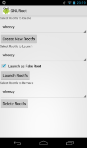
3. Once installed, just follow the steps to launch the Rootfs (Wheezy) as Fake Root. You will see a bash prompt, from which you can access a complete linux directory tree. This is the same as if you were in a computer (however, if you aren’t root you won’t be able to access the directories via your file browser from Android)

4. Now, we just have to update and upgrade:

apt-get update
apt-get upgrade

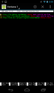
5. Then, update the sources.list file. We don’t have any graphical text editor (like gedit or kate)… but we have nano!:

nano /etc/apt/sources.list

Using the volume up + «W/S/A/D» you can move between the lines. Or alternatively, you can install a convenient keyboard with arrow buttons, like Hacker’s Keyboard! (thanks to JTT!)

Following instructions from CRAN, I added the following line to sources.list:

deb http://<favorite-cran-mirror>/bin/linux/debian wheezy-cran3/

Exit saving changes. But before «update and upgrade» again, don’t forget to add the key for the repository running the following:

apt-key adv --keyserver keys.gnupg.net --recv-key 381BA480

5. Update and upgrade…. voilà!

apt-get update
apt-get upgrade
apt-get install r-base r-base-dev

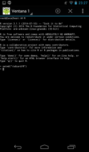
6. Now, you only have to run R just like in any bash console:

R GRAPHS

With this method you only have a prompt, without any graphical interface. ¿How do I make and see plots here?. If R runs from «inside» Android one option is to connect your Linux to an X-server app (thanks, J. Liebig). However, due to memory issues, I couldn’t put in practice this idea and see what happens. Try at your own risk! 🙂

Fortunately, there’s always possible to print R graphs in various formats, with the inconvenient that you have to browse to the plot’s location in Android -every time you need to check the output.

setwd("/sdcard")
data(cars)
pdf("cars.pdf")
plot(cars)
dev.off()

Here I leave a small script to begin playing with R on Android. Hope you enjoy it!

	###########################################
	### COMMANDS TO START WITH R ON ANDROID ###
	###########################################
	# Under GNU-GPL license

	# R in Android installed via the apps "GNURoot" and "GNURoot Wheezy", and sources.list updated with the newest CRAN repositories.
	# I strongly recommend to set the working directory of R to a folder that can be accessed from Android such as /sdcard

	setwd("/sdcard/R")

	# Just copy and paste the following commands, and press ENTER to see the results.
	# You can recycle these commands to make new ones suitable for your own data!
	# Note: the lines of text preceeded by "#" are considered comments, and they are not executed even if they are pasted.


	# Let's begin with real data:

	setwd("/sdcard/R")

	var0 <- c(64,76,66,47,72,82,66,58,64,69,80,57,66,63,71,55,57,71,45,77,69,61,47,55,59,45,61,56,68,74,55,71,72,64,52,62,69,53,76,62,65,54,73,79,74,38,61,73,75,71,74,52,48,45,65,59,79,78,82,61,70,73,68,76,71,65,78,65,80,69,73,70,80,50,67,70,63,68,70,37,73,68,53,73,79,76,68,80,79,78,75,82,72,77,75,66,72,66,66,58,70,71,69,81,74,45,73,81,71,76,79,80,72,64,81,79,74,69,75,56,62,60,83,55,74,47,70,59,47,81,73,59,74,70,69,81,29,77,72,78,68,60,65,83,66,76,68,80,82,79,74,74,22,62,81,75,75,44,72,75,72,77,76,67,70,76,42,56,76,84,75,76,83,73,63,50,78,70,79,74,59,54,74,68,72,82,69,48,64,48,78,62,87,79,65,70,85,80,79,72,71,77,76,79,76,81,82,70,65,79,76,83,75,63,52,80,86,63,68,69,78,82,74,86,69,85,72,64,57,74,78,22,77,64,63,51,74,71,71,47,63,66,73,43,72,75,81,40,56,71,77,77,71,69,68,58,64,76,73,81,73,81,59,68,57,62,66,76,66,47,72,82,66,58,64,69,80,57,66,63,71,55,57,71,45,77,69,61,47,55,59,45,61,56,68,74,52,71,72,64,52,62,69,53,76,62,65,54,73,79,74,38,61,73,75,71,75,82,72,77,75,66,72,66,66,58,81,74,45,73,81,71,76,79,80,72,64,81,
	79,74,69,75,56,62,60,83,55,74,47,70,59,47,81,73,59,74,70,69,81,29,77,72,78,68,60,65,83,66,76,68,80,82,79,74,74,22,62,81,75,75,44,72,75,72,77,76,67,70,76,42,56,76,84,75,76,83,73,63)

	var1 <- c("1","2","1","2","1","1","1","1","1","1","1","1","1","1","1","2","2","1","1","1","2","1","2","1","1","1","1","1","1","1","2","2","1","2","1","1","1","1","1","1","2","1","1","1","1","1","1","2","2","1","2","1","2","2","1","1","1","2","1","2","2","2","2","2","1","1","1","1","1","1","1","1","2","1","1","1","2","1","1","1","1","2","1","1","1","1","1","2","1","2","1","1","1","1","1","1","1","2","1","1","1","2","1","1","2","1","1","2","2","2","1","2","1","2","1","1","1","1","2","2","2","2","2","1","1","1","1","2","2","1","1","1","1","1","1","2","1","1","2","1","2","1","1","1","1","1","2","1","1","1","1","1","2","1","1","2","1","2","1","1","1","1","1","2","1","2","2","1","2","2","1","1","1","1","1","2","2","1","1","1","2","1","2","1","1","1","1","1","1","1","1","1","1","2","1","1","1","2","2","1","2","1","1","1","1","2","1","1","1","1","1","1","2","2","1","1","1","1","2","1","1","1","1","2","1","2","1","1","2","1","1","1","1","1","2","2","1","1","1","1","1","1","1","1","1","2","1","2","1","1","1","2","1",
	"2","2","1","1","1","1","1","1","1","1","1","1","2","1","2","1","1","1","1","2","1","1","1","2","1","2","2","1","1","1","1","2","1","1","1","1","1","1","1","1","1","1","1","2","1","1","1","2","1","1","1","2","2","1","1","2","2","1","1","1","2","1","1","1","1","1","2","1","1","1","1","1","2","1","2","2","1","1","1","1","1","2","1","2","1","1","1","1","1","1","2","1","2","1","1","1","1","1","1","2","2","1","1","2","1","2","2","1","2","2","1","2","2","2","1","2","1","2","2","1","1","1","1","1","1","1","1","1","2","2","1","1","2","2","2","1","2","2","2","2","1","2","1","1","2")

	var2 <- c("0","1","0","0","0","0","0","0","0","0","1","0","0","0","0","0","0","0","1","0","1","0","0","0","1","1","0","0","0","0","0","0","0","0","0","0","0","0","0","0","1","0","0","0","0","0","0","0","0","0","0","0","0","0","1","1","0","0","1","1","0","0","0","0","1","0","1","1","0","0","0","0","0","0","0","0","0","1","0","0","1","0","0","1","1","0","0","0","0","1","1","1","1","0","0","1","0","0","0","0","1","0","1","0","0","0","0","0","0","0","1","0","1","0","0","1","1","1","0","1","0","0","0","0","0","0","0","0","0","0","0","0","0","0","0","0","0","0","0","0","0","1","1","1","1","1","0","0","1","1","0","0","0","0","1","0","1","0","0","0","0","1","0","1","1","0","0","0","0","0","1","0","0","0","1","0","0","0","0","0","0","1","0","1","0","0","0","0","0","1","0","0","0","0","1","0","0","1","0","0","0","0","0","0","0","1","1","1","0","0","1","0","1","0","1","0","0","1","0","0","0","1","0","0","1","1","0","0","0","0","1","0","1","1","0","1","1","1","0","0","0","0","0","1","0","1","0","0","0","0","1","0","0",
	"0","0","0","0","0","1","0","0","0","1","0","1","0","0","0","1","0","0","1","0","0","0","0","0","0","0","0","0","0","0","0","0","0","0","0","0","0","0","0","0","0","0","0","0","0","0","0","0","0","0","0","0","0","0","0","0","0","0","0","0","0","0","0","0","0","0","0","0","0","0","0","0","0","0","0","0","1","0","0","0","0","0","1","0","0","0","0","0","0","0","0","0","0","0","0","1","0","0","1","0","0","0","0","0","1","1","0","1","0","0","1","0","0","0","0","0","0","0","0","1","0","0","0","1","0","0","0","0","1","0","0","1","0","0","0","0","0","0","0","0","0","0","0","0","0")

	mydatab <- data.frame(var0,var1,var2) # joins the vectors into a data frame

	# Global summary of my data.
	summary(mydatab)

	# Save the data.frame:
	save(mydatab, file="mydatab.RData")

	# Now we will print a plot using the pdf() function!
	pdf("myplotr.pdf")
	hist(mydatab$var0, breaks=30)
	dev.off()

view raw

RStartAndroid.R

hosted with ❤ by GitHub

Using gdata, for MS Windows users

Posted on May 18, 2013 por mareviv

Responder

I use both GNU-Linux and Windows systems on a regular basis… so I’m aware of the advantages (more for GNU-Linux in my case) and disadvantages of both.

Recently I needed to analyse a database from a remote location, an Excel (*xlsx) file.

The problem was that I couldn’t put my gdata library to work… some weird errors about a missing Perl interpreter… just needed to install one. Based on this tutorial in CRAN, I downloaded ActivePerl.

Then, I followed the instructions to install it, leaving the default options. The program sets the PATH to the interpreter, so R can finally find Perl…

Just start then a R session… Done!